

The Minimum Commitment Threshold
AWS commitments are one of the largest savings levers in an AWS estate, but few teams have a repeatable way to set a Minimum Commitment Threshold, the safe floor for what you can actually reserve.. The mechanism is simple: commit to a level of usage for one or three years through Savings Plans or Reserved Instances, and AWS gives you a discount in exchange.
The hard part is not understanding the product. The hard part is answering one question safely:
How much can we commit without turning savings into waste?
AWS gives you Savings Plans recommendations, but not an auditable model for answering that question. Most teams fill the gap with intuition, fear, or last quarter's purchase amount. They end up either under-committed, leaving savings untouched, or over-committed, paying for usage they cannot fill.
The missing concept is the Minimum Commitment Threshold: the conservative level of on-demand equivalent spend that your usage shape can support as a commitment in every hour.
This post gives the simple version of the model. It avoids the advanced product-tiering problem and focuses on the core idea: commitments are safe when your usage is stable enough to fill them, and the right way to find that stable level is by looking at your hourly spend distribution.
To keep this concrete, this series follows one company: Alpenglow Outfitters, a ~450-person outdoor-gear retailer, AWS-native, running roughly $8M/year (precisely $7.884M) of commitment-eligible, on-demand equivalent (ODE) compute spend across three business units. Every number below is derived from Alpenglow's usage shape — substitute your own and the method is identical.
What a Commitment Actually Buys You
A Savings Plan or Reserved Instance is a promise to AWS: you agree to pay for a certain amount of usage every hour for the term of the commitment. AWS discounts that usage in exchange for the guarantee.
The important part is the guarantee.
You pay whether the usage appears or not. If the commitment is filled, the discount is real savings. If the commitment is not filled, the unused portion becomes breakage. At enough breakage, the discount can disappear entirely or turn negative.
There is also a translation issue. AWS bills commitments in post-discount dollars, while your usage is usually easier to reason about in on-demand equivalent dollars. If a Compute Savings Plan gives a 31% discount, then $69/hour of committed spend covers $100/hour of on-demand equivalent usage. The commitment amount and the usage level are not expressed in the same units.
For planning, use on-demand equivalent spend. Ask: how much eligible usage, measured as if it were still on-demand, is stable enough to fill a commitment every hour of the year?
That stable amount is the Minimum Commitment Threshold.
Fifty shades of commitment
Not all AWS spend belongs in the same commitment pool.
Compute, Database, and SageMaker each have their own eligible usage and their own commitment products. Even inside Compute, different products can overlap. EC2 usage can be eligible for more than one commitment type. Lambda and Fargate are different from EC2. Database commitments behave differently again.
That matters, but it is not the first concept to learn.
For a simple implementation, treat the estate as a small set of commitment-eligible segments:
- Compute eligible ODE
- Database eligible ODE
- SageMaker eligible ODE
That maps cleanly onto Alpenglow's estate: EKS and Fargate compute, an RDS/Aurora database fleet, and SageMaker training and inference inside Data & ML.
Compute the hourly distribution and minimum threshold separately for each exclusive commitment segment. Then roll the segment levels up into one total Minimum Commitment Threshold.
The advanced version is about assigning each dollar to exactly one product tier before calculating the minimum threshold, so you do not double-count overlapping eligibility pools. That is important for a production-grade model. But the core diagnostic does not require starting there.
The first-order question is simpler: for each major eligible segment, how much spend is stable enough to commit?
The Problem Is Shape, Not Average Spend
A common error is to start with average spend.
If a workload averages $100/hour over the month, it is tempting to think a $100/hour commitment is safe. But averages hide the only thing that matters: whether usage is present in each hour when the commitment bill arrives.
Alpenglow's business units make this concrete. Two of them have different averages and opposite hourly profiles:
- Storefront (web/API, checkout) is day-peaking: ~$650/hour during business hours, ~$250/hour overnight, averaging $450/hour.
- Data & ML (batch pipelines, recommendation training and inference) is night-peaking: ~$450/hour overnight, ~$150/hour daytime, averaging $300/hour.
Each curve alone is jagged — a commitment sized to either BU's own average sits unfilled for part of every day. But their peaks fall in opposite hours, so the combined estate curve is far smoother than either unit alone. That whole-estate shape, not any single average, sets how much Alpenglow can safely commit.
That is why the Minimum Commitment Threshold is a distribution problem. You are not trying to forecast the average. You are trying to find the level of usage that appears often enough, hour by hour, to make the commitment economically rational.
Take Storefront as that one piece. Gather its historical on-demand equivalent spend across a full seasonal window. The result is a distribution showing how its spend behaves at each hour of the day, best visualized as a box plot below. In that context, the Storefront-local Minimum Commitment Threshold is the floor of all hours, indicated by the dotted line.
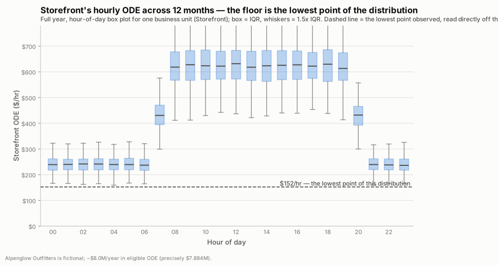
Storefront's hourly ODE across 12 months. Its Minimum Commitment Threshold is the lowest point of this distribution: $152/hr — read directly off the chart, not asserted.
The same non-overlap applies across business units: Storefront, Data & ML, and Marketplace & Logistics never bottom out at the same hour, so their floors don't simply add to a combined minimum — here's what the combined estate actually looks like:
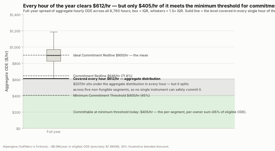
The combined estate covers $612/hr in every single hour of the year. Yet $612/hr still isn't the Minimum Commitment Threshold: no single AWS instrument covers a business's whole estate. Real commitments split across five non-fungible products — Reserved Instances, several kinds of Savings Plans — which lowers the real committable number further. Work through that breakdown and the real Minimum Commitment Threshold comes out to $405/hr (see the ladder below); Blog 3.5 has the full math.
Alpenglow's combined hourly ODE across all 8,760 hours of the year. The Minimum Commitment Threshold ($405/hr) sits well below what the combined estate covers every hour ($612/hr) — the gap is real, but it isn't purchasable as one instrument.
Use at least one full seasonal cycle. Twelve months is the minimum. Three years is better if the business has meaningful annual patterns. Alpenglow's shape makes the point: its Q4 holiday peak runs about 40% above the May trough, with a smaller ~15% summer camping bump, so a window that misses Q4 would anchor the minimum threshold to a level that only holds for part of the year.
The Percentile Is Not Arbitrary
The key move is to draw the right percentile line on those hourly distributions.
This percentile should not be a guess. It comes from the discount rate.
Suppose a No Upfront commitment gives a 31% discount. For a marginal extra dollar of commitment:
- When usage fills that dollar, you save 31 cents.
- When usage does not fill that dollar, you lose the 69 cents you still paid.
The break-even point is where those outcomes balance. For a No Upfront product with a D% discount, the marginal break-even level is the pD level of the usage distribution.
So a 31% discount maps to p31. A 50% discount maps to p50. Higher-discount products can rationally reach higher into the distribution because the upside on filled hours is larger.
(Discount rates in this post are illustrative round numbers. API-verified market rates — Compute SP 1y NU 26.5% / FU 31.4%; 3y NU 49.3% / FU 54.0% (us-east-1, July 2026) — are tabulated in the payment-option post; recompute the percentiles from your actual rates.)
That is the economic intuition behind the Commitment Redline:
The Commitment Redline is the highest level of eligible ODE spend that still sits at or below the product's marginal break-even percentile across the hourly distribution. The Minimum Commitment Threshold sits below it: the level covered in every hour, utilized 100% by construction.
The Ideal Commitment Redline and Minimum Commitment Rate
The Minimum Commitment Threshold tells you the conservative level your current usage shape supports.
But there is a second number worth computing: the Ideal Commitment Redline.
Imagine eligible ODE were perfectly flat over time. No peaks. No troughs. No business-unit fragmentation. No overnight valleys. Every hour carries the same amount of eligible usage.
In that ideal case, the maximum structurally fillable commitment level is simply:
In practical terms, this is the average hourly eligible ODE.
For Alpenglow, that is $7.884M/year ÷ 8,760 hours = $900/hour — the same figure you get by summing the three BU averages ($450 + $300 + $150).
This is not a purchase recommendation. It is a theoretical shape cap — a benchmark, never a target. No orchestration strategy can make the Minimum Commitment Threshold exceed the eligible usage itself. The best possible shape is a flat line.
That makes the ratio useful:
This ratio measures how much of the ideal your usage shape actually makes safely committable.
If the ratio is low, your estate has a lot of eligible spend, but the shape is preventing you from committing much of it safely. The cause may be workload variance, business-unit isolation, poor timing of flexible jobs, disabled sharing, or priority rules that prevent commitments from flowing to the most stable usage.
If the ratio is high, your estate is already well orchestrated. Usage is pooled, smooth, and easier to commit. The next improvement may come less from reshaping the estate and more from better acquisition execution.
Alpenglow sits in the low-to-middle band. Because each business unit buys its own commitments in isolation, its Minimum Commitment Threshold is about 45% of eligible ODE — a Minimum Commitment Rate of roughly 0.45 against the $900/hour Ideal Commitment Redline. Pool those commitments at the payer so Storefront's daytime peak and Data & ML's overnight peak offset inside one curve, and the minimum threshold rises to about 60.6% ($545/hour) — a Minimum Commitment Rate of 0.61. That 0.45 → 0.61 gap is pure orchestration gain; a later post in the series puts a dollar figure on it.
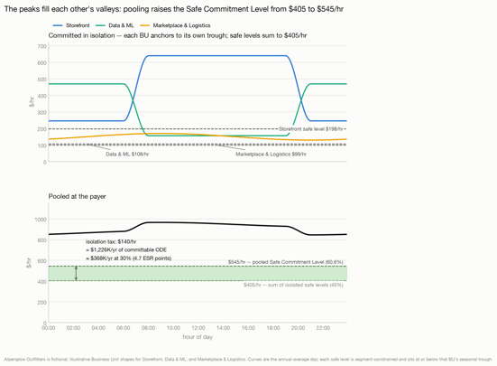
This is the missing distinction: the Minimum Commitment Threshold tells you how much is safely committable now. The Ideal Commitment Redline tells you how much could be committable if the usage shape were perfectly flat.
Orchestration work closes that gap: it pushes the Commitment Redline toward the Ideal Commitment Redline and pulls the Minimum Commitment Threshold up behind it. The distance between the redline and the ideal is the Orchestration Headroom.
The Commitment Ladder
Once you have the Minimum Commitment Threshold, the Commitment Redline, and the Ideal Commitment Redline, you can put the whole strategy on one line.
Start at 0. End at the Ideal Commitment Redline. Then place the important markers on the line:
- Current covered ODE % (with ESR as the derived outcome)
- Minimum Commitment Threshold
- Commitment Redline
- Ideal Commitment Redline
- Meaningful product percentiles, such as p27 for a 1-year No Upfront Compute SP's ~26.5% discount rate, then higher milestones such as p50 or p61 for longer or higher-discount plans
For Alpenglow, the line runs from 0 to $900/hour, with today's markers at covered ODE 35%, Minimum Commitment Threshold 45%, Commitment Redline 71.8% ($646/hour), and Ideal Commitment Redline 100% ($900/hour), all as a share of eligible ODE — covered 35% at a ~30% blended discount ≈ ESR 10.5%. The covered position sitting below the minimum threshold is the tell: there is an execution gap to close up to the Minimum Commitment Threshold before taking on any risk above it.
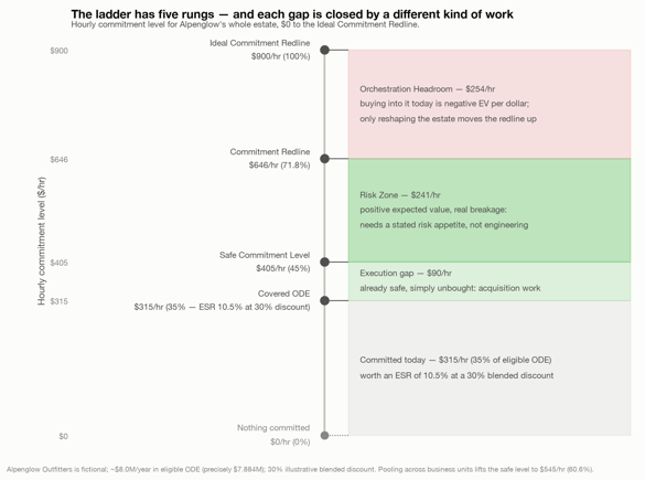
The Commitment Ladder from $0 to $900/hr
One line shows the whole strategy: covered ODE ($315/hr), the Minimum Commitment Threshold ($405/hr), the pooled potential ($545/hr), and the $900/hr shape cap.
From 0 to the Minimum Commitment Threshold, you are closing the conservative gap. This is the low-risk zone. If your covered position sits below the minimum threshold, the first job is usually acquisition: buy the right commitments, fix sharing, clean up timing, and reduce avoidable under-commitment.
At the Minimum Commitment Threshold, you have reached the conservative minimum reference point.
Above the Minimum Commitment Threshold, you are in the Risk Zone. That does not mean stop. It means each additional layer needs a stated thesis, justified by the percentile math. A 1-year No Upfront product may justify reaching to p27. A longer or higher-discount plan may justify reaching higher because the savings on filled hours are larger. The sequence should be deliberate: fill the lower-risk layer first, then stack higher-risk layers only when the expected value remains positive.
The Ideal Commitment Redline is the outer structural boundary. If your covered position is below the Minimum Commitment Threshold, you have an execution gap. If the Commitment Redline is far below the Ideal Commitment Redline, you have an orchestration gap. If your covered position is above the Minimum Commitment Threshold, you have a risk position that needs to be modeled explicitly.
The Risk Zone Above the Minimum Threshold
The Minimum Commitment Threshold is not an absolute ceiling.
It is the conservative minimum reference point. You can commit above it, and most of the time that is the right decision. But above the minimum threshold, you are no longer making a low-risk decision. You are making a risk/reward decision.
For any candidate commitment in the Risk Zone — between the Minimum Commitment Threshold and the Commitment Redline — estimate:
If expected value is still positive, committing above the minimum threshold can be rational. The extra savings on filled hours outweigh the expected breakage in unfilled hours.
If expected value is negative — guaranteed for every dollar above the Commitment Redline, the Over-Commitment Zone — the extra commitment is no longer a savings strategy. It is a bet. Maybe the company is growing. Maybe workloads will be shifted. Maybe business units will be pooled. Maybe automation will track the floor more closely. Those can be good bets, but they should be named as bets.
This is where the Ideal Commitment Redline becomes useful. If you are above the minimum threshold but still below the Ideal Commitment Redline, the risk is partly a question of orchestration: can the company reshape usage fast enough to make the higher commitment safe?
Two Ways to Raise the Minimum Threshold
Once you compute the minimum threshold, the next question is obvious: how do you raise it?
The short answer is: reduce variance in eligible usage.
The two most common levers are pooling and scheduling.
Pooling means commitments are shared across heterogeneous usage patterns instead of trapped inside individual accounts or business units. Alpenglow is the textbook case: Storefront peaks during business hours while Data & ML peaks overnight, so sharing their commitments at the payer produces an aggregate curve smoother than either alone. A smoother curve has a higher minimum threshold.
Scheduling means moving flexible workloads into valleys. Batch jobs, data pipelines, training workloads, and non-urgent compute can sometimes be shifted away from peak hours into troughs. That raises the low parts of the curve and makes more spend safely committable.
Other levers include growth-aware micro-commitments, fixing sharing configuration, and removing priority rules that allocate commitment benefits according to metadata rather than economic value.
The details vary by estate. The principle does not: a higher minimum threshold comes from a flatter, more aggregated, better-orchestrated usage shape. Orchestration work pushes the Commitment Redline toward the Ideal Commitment Redline and pulls the Minimum Commitment Threshold up behind it.
Why AWS Tooling Does Not Show This
AWS surfaces utilization and coverage because they are easy to compute after commitments exist.
Utilization tells you whether the commitments you bought were filled. Coverage tells you how much usage received a commitment discount.
Neither tells you what you should have bought.
Neither shows the hourly distribution. Neither computes the Minimum Commitment Threshold. Neither tells you how far your current shape is from the Ideal Commitment Redline.
That is the missing model.
Without it, a recommendation is hard to inspect. If AWS suggests a purchase, you cannot easily see the seasonal window, the percentile assumption, the breakage risk, or the structural headroom behind the number.
With it, the conversation changes. You can explain why a commitment level is safe, why a higher level is risk-taking, and which operational changes would increase the minimum threshold.
What to Do With This
The simple workflow is:
- Define the major commitment-eligible segments: Compute, Database, SageMaker.
- Pull hourly ODE spend for each segment over a 12-36 month window.
- Build hour-of-day distributions for each segment.
- Choose the product discount rate and draw the corresponding break-even percentile line — this sets the Commitment Redline.
- Compute the Minimum Commitment Threshold for each segment.
- Roll segment levels into one total Minimum Commitment Threshold.
- Compute the Ideal Commitment Redline as average hourly eligible ODE.
- Compare the Minimum Commitment Rate (Minimum Commitment Threshold / Ideal Commitment Redline) to measure how much of the ideal your usage shape actually makes safely committable.
- Treat commitments above the minimum threshold as explicit risk/reward decisions, not risk-free savings.
The Minimum Commitment Threshold tells you what is safe now. The Ideal Commitment Redline tells you what the estate could support if usage were perfectly orchestrated. The gap between them tells you whether the next structural savings point should come from pooling, smoothing, scheduling, sharing configuration, or accepting modeled risk above the minimum threshold.
What the Minimum Commitment Threshold does not tell you is how efficiently you are actually acquiring against it. That is a second metric: Effective Savings Rate. It will be the subject of the next post.